library(INLA)
library(tidyverse)Simulation study
In the vignette Simulation example, we simulate a single data set with Berkson error, classical error and missing data, and then fit a measurement error model to adjust for these errors. In this simulation study, we do the exact same steps, but repeated on 100 simulated data sets instead of just one, to ensure that the results are not an artifact of one particular data set. This vignette consists of mostly just code, for detailed explanations on the steps taken in the analysis, please refer to Simulation example.
Setting up functions
Function for simulating data
simulate_data <- function(n){
  # Covariate without error:
  z <- rnorm(n, mean = 0, sd = 1)

  # Berkson error:
  u_b <- rnorm(n)
  r <- rnorm(n, mean = 1 + 2*z, sd = 1)
  x <- r + u_b

  # Response:
  y <- 1 + 2*x + 2*z + rnorm(n)

  # Classical error:
  u_c <- rnorm(n)
  w <- r + u_c

  # Missingness:
  m_pred <- -1.5 - 0.5*z # MAR. This gives a mean probability of missing of ca 0.2.
  # m_pred <- -1.5 - 0.5*x # MNAR
  m_prob <- exp(m_pred)/(1 + exp(m_pred))
  m_index <- as.logical(rbinom(n, 1, prob = m_prob)) # MAR/MNAR
  # m_index <- sample(1:n, 0.2*n, replace = FALSE) # MCAR
  w[m_index] <- NA

  simulated_data <- data.frame(y = y, w = w, z = z, x = x)
  return(simulated_data)
}
Functions for setting up the model matrices
# Make matrix for ME model
make_matrix_ME <- function(data){
  n <- nrow(data)

  y <- data$y
  w <- data$w
  z <- data$z

  Y <- matrix(NA, 4*n, 4)

  Y[1:n, 1] <- y                 # Regression model of interest response
  Y[n+(1:n), 2] <- rep(0, n)     # Berkson error model response
  Y[2*n+(1:n), 3] <- w           # Classical error model response
  Y[3*n+(1:n), 4] <- rep(0, n)   # Imputation model response

  beta.0 <- c(rep(1, n), rep(NA, 3*n))
  beta.x <- c(1:n, rep(NA, 3*n))
  beta.z <- c(z, rep(NA, 3*n))

  id.x <- c(rep(NA, n), 1:n, rep(NA, n), rep(NA, n))
  weight.x <- c(rep(NA, n), rep(-1, n), rep(NA, n), rep(NA, n))

  id.r <- c(rep(NA, n), 1:n, 1:n, 1:n)
  weight.r <- c(rep(NA, n), rep(1, n), rep(1, n), rep(-1, n))

  alpha.0 = c(rep(NA, 3*n), rep(1, n))
  alpha.z = c(rep(NA, 3*n), z)

  dd_adj <- list(Y = Y,
                       beta.0 = beta.0,
                       beta.x = beta.x,
                       beta.z = beta.z,
                       id.x = id.x,
                       weight.x = weight.x,
                       id.r = id.r,
                       weight.r = weight.r,
                       alpha.0 = alpha.0,
                       alpha.z = alpha.z)

  return(dd_adj)
}

# Make matrix for naive model
make_matrix_naive <- function(data){
  y <- data$y
  w <- data$w
  z <- data$z

  # Naive model
  dd_naive <- list(Y = y,
                         beta.0 = rep(1, nrow(data)),
                         beta.x = w,
                         beta.z = z)
  return(dd_naive)
}

# Make matrix for model using the unobserved variable
make_matrix_true <- function(data){
  y <- data$y
  x <- data$x
  z <- data$z
  # True model
  dd_naive <- list(Y = y,
                         beta.0 = rep(1, nrow(data)),
                         beta.x = x,
                         beta.z = z)
}
Function for fitting the ME model
# Fit ME model
fit_model_ME <- function(data_matrix) {
  # Priors for model of interest coefficients
  prior.beta <- c(0, 1/1000) # N(0, 10^3)

  # Priors for exposure model coefficients
  prior.alpha <- c(0, 1/10000) # N(0, 10^4)

  # Priors for y, measurement error and true x-value precision
  prior.prec.y <- c(10, 9) # Gamma(10, 9)
  prior.prec.u_b <- c(10, 9) # Gamma(10, 9)
  prior.prec.u_c <- c(10, 9) # Gamma(10, 9)
  prior.prec.r <- c(10, 9) # Gamma(10, 9)

  # Initial values
  prec.y <- 1
  prec.u_b <- 1
  prec.u_c <- 1
  prec.r <- 1

  # Formula
  formula = Y ~ - 1 + beta.0 + beta.z +
    f(beta.x, copy = "id.x",
      hyper = list(beta = list(param = prior.beta, fixed = FALSE))) +
    f(id.x, weight.x, model = "iid", values = 1:n,
      hyper = list(prec = list(initial = -15, fixed = TRUE))) +
    f(id.r, weight.r, model="iid", values = 1:n,
      hyper = list(prec = list(initial = -15, fixed = TRUE))) +
    alpha.0 + alpha.z

  # Fit model
  model <- inla(formula,
                data = data_matrix,
                family = c("gaussian", "gaussian", "gaussian", "gaussian"),
                control.family = list(
                  list(hyper = list(prec = list(initial = log(prec.y),
                                                param = prior.prec.y,
                                                fixed = FALSE))),
                  list(hyper = list(prec = list(initial = log(prec.u_b),
                                                param = prior.prec.u_b,
                                                fixed = FALSE))),
                  list(hyper = list(prec = list(initial = log(prec.u_c),
                                                param = prior.prec.u_c,
                                                fixed = FALSE))),
                  list(hyper = list(prec = list(initial = log(prec.r),
                                                param = prior.prec.r,
                                                fixed = FALSE)))),
                control.predictor = list(compute = TRUE),
                control.fixed = list(
                  mean = list(
                    beta.0 = prior.beta[1],
                    beta.z = prior.beta[1],
                    alpha.0 = prior.alpha[1],
                    alpha.z = prior.alpha[1]),
                  prec = list(
                    beta.0 = prior.beta[2],
                    beta.z = prior.beta[2],
                    alpha.0 = prior.alpha[2],
                    alpha.z = prior.alpha[2])
    )
  )
}
Function for fitting the true/naive model
The same function can be used to fit the naive model (y ~ w + z) and the best-case model (y ~ x + z) since they simply differ in the variable that is inputted (w versus x).
fit_model_naive_true <- function(data_matrix){
  # Priors for model of interest coefficients
  prior.beta <- c(0, 1/1000) # N(0, 10^3)

  # Priors for y, measurement error and true x-value precision
  prior.prec.y <- c(10, 9) # Gamma(10, 9)

  # Initial values
  prec.y <- 1

  # Formula
  formula <- Y ~ beta.0 - 1 + beta.x + beta.z

  # Fit model
  model <- inla(formula,
                data = data_matrix,
                family = c("gaussian"),
                control.family = list(
                  list(hyper = list(prec = list(initial = log(prec.y),
                                                param = prior.prec.y,
                                                fixed = FALSE)))),
                control.fixed = list(
                  mean = list(
                    beta.0 = prior.beta[1],
                    beta.z = prior.beta[1],
                    beta.x = prior.beta[1]),
                  prec = list(
                    beta.0 = prior.beta[2],
                    beta.z = prior.beta[2],
                    beta.x = prior.beta[2])
    )
  )
}
Fitting the model for each data set
We simulate 100 data sets and fit the model that accounts for measurement error and missing data, and then save the posterior means for the intercept ans slopes.
Note that this chunk may take a while to run.
set.seed(1)

# Number of iterations
niter <- 100

# Data frames to store the results
results_ME <- data.frame(matrix(NA, nrow=niter, ncol=5))
names(results_ME) <- c("beta.0", "beta.x", "beta.z", "alpha.0", "alpha.z")

results_naive <- data.frame(matrix(NA, nrow=niter, ncol=3))
names(results_naive) <- c("beta.0", "beta.x", "beta.z")

results_true <- data.frame(matrix(NA, nrow=niter, ncol=3))
names(results_true) <- c("beta.0", "beta.x", "beta.z")

for(i in 1:niter){
  n <- 1000
  data <- simulate_data(n)

  # ME model
  matrix_ME <- make_matrix_ME(data)
  model_ME <- fit_model_ME(matrix_ME)

  # Naive model
  matrix_naive <- make_matrix_naive(data)
  model_naive <- fit_model_naive_true(matrix_naive)

  # True model
  matrix_true <- make_matrix_true(data)
  model_true <- fit_model_naive_true(matrix_true)

  results_ME[i, c("beta.0", "beta.z",
                  "alpha.0", "alpha.z")] <- t(model_ME$summary.fixed["mean"])
  results_ME[i, "beta.x"] <- model_ME$summary.hyperpar["Beta for beta.x", "mean"]

  results_naive[i, c("beta.0", "beta.x", "beta.z")] <- t(model_naive$summary.fixed["mean"])

  results_true[i, c("beta.0", "beta.x", "beta.z")] <- t(model_true$summary.fixed["mean"])

}
Results
saveRDS(joint_results, file = "results/simulation_results.rds")library(colorspace)
library(showtext)
showtext_auto()
# Colors
col_bgr <- "white" #"#fbf9f4"
col_text <- "#191919"
color_pal <- c("#004488", "#DDAA33", "#BB5566")
# Loading fonts
f1 <- "Open Sans"
font_add_google(name = f1, family = f1)
font_size <- 20
# Plot theme
theme_model_summary <- theme_minimal(base_size = font_size, base_family = f1) +
theme(
axis.title.y = element_blank(),
axis.title.x = element_text(size = 0.7*font_size, color = col_text, family = f1),
axis.text.y = element_text(size = 0.6*font_size, color = col_text, family = f1),
axis.text.x = element_text(size = 0.4*font_size, color = col_text, family = f1,
margin = margin(0, 0, 1, 0)),
axis.ticks = element_blank(),
legend.title = element_blank(),
panel.background = element_rect(fill = col_bgr, color = col_bgr),
plot.background = element_rect(fill = col_bgr, color = col_bgr),
legend.position = "none",
strip.placement = "outside",
strip.text = element_text(color = col_text),
panel.grid.major.y = element_blank(),
panel.grid.minor.y = element_blank(),
panel.border = element_rect(color = "grey65", fill = NA, linewidth = 1), #
plot.title.position = "plot",
axis.line.x = element_line(linewidth = 1, color = "grey65"),#
plot.margin = margin(rep(15, 4))
)
ggplot(simulation_results, aes(x = value, y = model, color = model)) +
# Invisible points to set limits
#geom_point(aes(x = upper), alpha = 0) +
#geom_point(aes(x = lower), alpha = 0) +
# Line going up from best case model
geom_segment(aes(x = true_value, xend = true_value),
y = "Best case model", yend = Inf,
color = "grey30", linetype = "dotted", linewidth = 0.8) +
# Points for each run
geom_point(aes(fill = stage(model, after_scale = lighten(fill, 0.4))),
alpha = 0.7, size = 1.5, pch = 21, stroke = 0,
position = position_jitterdodge(jitter.width = 0.8, seed = 1)) +
# Error lines
stat_summary(geom = "linerange",
fun.min = function(z) {quantile(z, 0.025)},
fun.max = function(z) {quantile(z, 0.975)},
position = position_dodge(width = 0.75),
linewidth = 1.3) +
# Point for mean
geom_point(aes(x = mean), size = 3) +
# Numeric text at mean
geom_text(aes(x = mean,
y = model,
label = format(round(mean, digits=2), nsmall = 2)),
vjust = -1.5, family = f1, size = 5, color = col_text) +
# Color for point and line
scale_color_manual(values = color_pal) +
scale_fill_manual(values = color_pal) +
# One plot for each variable
facet_wrap(vars(variable),
nrow = 1,
labeller = label_parsed,
scales = "free_x") +
# x-axis breaks
scale_x_continuous(breaks = seq(0, 4, 1)) +
# Lables
labs(x = "Posterior mean") +
# Add theme
theme_model_summary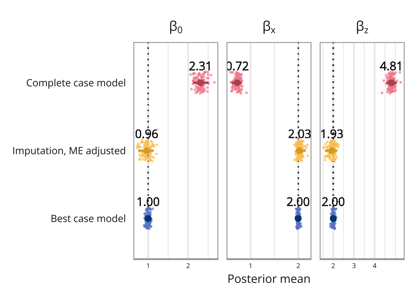
ggsave("figures/simulation_boxplot.pdf",
       width = 10, height = 4, dpi = 600)
ggsave("figures/simulation_boxplot.eps", width = 10, height = 4, dpi = 600,
       device = cairo_ps)