Influence of systolic blood pressure on coronary heart disease
Source:vignettes/Framingham_heart_study.Rmd
Framingham_heart_study.RmdIn this tutorial, we re-do the analysis from two previous
publications that use the same data set. The data set contains the heart
disease status for a number of patients, along with repeated
measurements of their systolic blood pressure and their smoking status.
The data is also included in the package, simply type
?framingham for more details.
head(framingham)
#>   disease         sbp1        sbp2 smoking         sbp
#> 1       0  0.043556319 -0.24144440       0 -0.09894404
#> 2       0 -0.088249125 -0.03871185       1 -0.06348049
#> 3       0  0.063634980  0.02971774       1  0.04667636
#> 4       0 -0.331791943 -0.44704230       1 -0.38941712
#> 5       0  0.006502333 -0.09760337       1 -0.04555052
#> 6       0  0.124884993  0.09793482       0  0.11140991
The two publications are Bayesian analysis of measurement error models using INLA, Muff et al (2015) and Reverse attenuation in interaction terms due to covariate measurement error, Muff & Keller (2015).
First example: A logistic regression model with repeated measurements
| Error types | Likelihood | Response | Covariate with error | Other covariate(s) |
|---|---|---|---|---|
| Classical | Binomial | disease |
sbp1, sbp2
|
smoking |
The data and model in this example was also used in Muff et al (2015), so more
information on the measurement error model can be found there. The model
is identical, this example just shows how it can be implemented in
inlamemi.
In this example, we fit a logistic regression model for whether or
not a patient has heart disease, using systolic blood pressure (SBP) and
smoking status as covariates. SBP is measured with error, but we have
repeated measurements, and so we would like to feed both measurements of
SBP into the model. This can be done easily in the inlamemi
package.
The formula for the main model of interest will be and the formula for the imputation model will be
In addition, we of course also have the classical measurement error model that describes the actual error in the SBP measurements, and since we have repeated measurements we actually have two: where are the measurement error terms.
We can then call the fit_inlamemi function directly with
the above formulas for the model of interest and imputation model. Also
note the repeated measurements argument, which must be set to
TRUE to ensure that the model is specified correctly. We
give the precision for the error term of the measurement error model a
prior, and the error term for the imputation model a prior. By default
in R-INLA, the fixed effects are given Gaussian priors with mean
and precision
.
We re-assign the precisions to be
,
but keep the means at 0 (therefore they are not specified in the
control.fixed argument).
framingham_model <- fit_inlamemi(formula_moi = disease ~ sbp + smoking,
                               formula_imp = sbp ~ smoking,
                               family_moi = "binomial",
                               data = framingham,
                               error_type = "classical",
                               repeated_observations = TRUE,
                               prior.prec.classical = c(100, 1),
                               prior.prec.imp = c(10, 1),
                               prior.beta.error = c(0, 0.01),
                               initial.prec.classical = 100,
                               initial.prec.imp = 10,
                               control.fixed = list(
                                 prec = list(beta.0 = 0.01,
                                             beta.smoking = 0.01,
                                             alpha.0 = 0.01,
                                             alpha.smoking = 0.01)))
Once the model is fit we can look at the summary.
summary(framingham_model)
#> Formula for model of interest:
#> disease ~ sbp + smoking
#>
#> Formula for imputation model:
#> sbp ~ smoking
#>
#> Error types:
#> [1] "classical"
#>
#> Fixed effects for model of interest:
#>                    mean        sd 0.025quant   0.5quant 0.975quant       mode
#> beta.0       -2.3615593 0.2704869  -2.893447 -2.3610439 -1.8325961 -2.3610384
#> beta.smoking  0.3993937 0.2994675  -0.187501  0.3992729  0.9869775  0.3992727
#>
#> Coefficient for variable with measurement error and/or missingness:
#>              mean        sd 0.025quant 0.5quant 0.975quant     mode
#> beta.sbp 1.897425 0.5598872  0.8404353 1.882702   3.043093 1.816999
#>
#> Fixed effects for imputation model:
#>                          mean         sd  0.025quant    0.5quant 0.975quant        mode
#> alpha.sbp.0        0.01454298 0.01858277 -0.02190736  0.01454298 0.05099333  0.01454298
#> alpha.sbp.smoking -0.01958476 0.02156433 -0.06188347 -0.01958476 0.02271395 -0.01958476
#>
#> Model hyperparameters (apart from beta.sbp):
#>                                       mean       sd 0.025quant 0.5quant 0.975quant     mode
#> Precision for sbp classical model 75.90178 3.690529   68.89246 75.81334   83.41982 75.63953
#> Precision for sbp imp model       19.89452 1.234087   17.55047 19.86501   22.40730 19.82463
plot(framingham_model)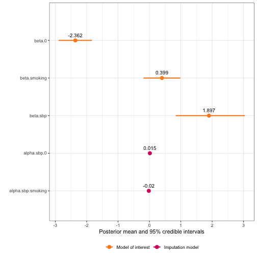
For a comparison, we can also fit a “naive” model, that is, a model that ignores the measurement error in SBP. For this model, we will take an average of the two SBP measurements and use that as the SBP variable.
framingham$sbp <- (framingham$sbp1 + framingham$sbp2)/2
naive_model <- inla(formula = disease ~ sbp + smoking,
                    family = "binomial",
                    data = framingham)
naive_model$summary.fixed
#>                   mean        sd 0.025quant   0.5quant 0.975quant       mode kld
#> (Intercept) -2.3547258 0.2692636 -2.8824728 -2.3547258 -1.8269788 -2.3547258   0
#> sbp          1.6686897 0.4937443  0.7009686  1.6686897  2.6364107  1.6686897   0
#> smoking      0.3972557 0.2992211 -0.1892069  0.3972557  0.9837183  0.3972557   0
Then we can compare the estimated coefficients from both models.
naive_result <- naive_model$summary.fixed
rownames(naive_result) <- c("beta.0", "beta.sbp", "beta.smoking")
naive_result$variable <- rownames(naive_result)
me_result <- rbind(summary(framingham_model)$moi_coef[1:6],
                   summary(framingham_model)$error_coef[1:6])
me_result$variable <- rownames(me_result)
results <- dplyr::bind_rows(naive = naive_result, me_adjusted = me_result, .id = "model")

ggplot(results, aes(x = mean, y = model, color = variable)) +
  geom_point() +
  geom_linerange(aes(xmin = `0.025quant`, xmax = `0.975quant`)) +
  facet_grid(~ variable, scales = "free_x") +
  theme_bw()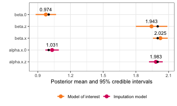
Second example: Heteroscedastic measurement error and interaction between error variable and error free variable
| Error types | Likelihood | Response | Covariate with error | Other covariate(s) |
|---|---|---|---|---|
| Classical (with interaction effects) | Binomial | disease |
sbp1, sbp2
|
smoking |
In this example, we artificially increase the measurement error for the smoking group in order to study a model with homoscedastic measurement error. The model in this example is identical to that in Muff & Keller (2015)
framingham2 <- framingham
n <- nrow(framingham2)

set.seed(1)
framingham2$sbp1 <- framingham$sbp1 +
  ifelse(framingham2$smoking == 1, rnorm(n, 0, 0.117), 0)
framingham2$sbp2 <- framingham$sbp2 +
  ifelse(framingham2$smoking == 1, rnorm(n, 0, 0.117), 0)

# Or:
#framingham2 <- read.table("../data-raw/fram_data_case2.txt", header=T)
#names(framingham2) <- c("disease", "sbp1", "sbp2", "smoking")

#framingham2$sbp <- (framingham2$sbp1 + framingham2$sbp2)/2
error_scaling <- c(1/(1+9*framingham2$smoking), 1/(1+9*framingham2$smoking))
# Homoscedastic ME modeled as homoscedastic ME (correct)
framingham_model2.1 <- fit_inlamemi(formula_moi = disease ~ sbp:smoking,
                               formula_imp = sbp ~ smoking,
                               family_moi = "binomial",
                               data = framingham,
                               error_type = "classical",
                               repeated_observations = TRUE,
                               prior.prec.classical = c(100, 1),
                               prior.prec.imp = c(10, 1),
                               prior.beta.error = c(0, 0.01),
                               initial.prec.classical = 100,
                               initial.prec.imp = 10,
                               control.fixed = list(
                                 prec = list(beta.0 = 0.01,
                                             beta.smoking = 0.01,
                                             alpha.0 = 0.01,
                                             alpha.smoking = 0.01)))

# Heteroscedastic ME modeled as heteroscedastic ME (correct)
framingham_model2.2 <- fit_inlamemi(formula_moi = disease ~ sbp:smoking,
                               formula_imp = sbp ~ smoking,
                               family_moi = "binomial",
                               data = framingham2,
                               error_type = "classical",
                               repeated_observations = TRUE,
                               classical_error_scaling = error_scaling,
                               prior.prec.classical = c(100, 1),
                               prior.prec.imp = c(10, 1),
                               prior.beta.error = c(0, 0.01),
                               initial.prec.classical = 100,
                               initial.prec.imp = 10,
                               control.fixed = list(
                                 prec = list(beta.0 = 0.01,
                                             beta.smoking = 0.01,
                                             alpha.0 = 0.01,
                                             alpha.smoking = 0.01)))

# Heteroscedastic ME modeled as homoscedastic ME (incorrect)
framingham_model2.3 <- fit_inlamemi(formula_moi = disease ~ sbp:smoking,
                               formula_imp = sbp ~ smoking,
                               family_moi = "binomial",
                               data = framingham2,
                               error_type = "classical",
                               repeated_observations = TRUE,
                               prior.prec.classical = c(100, 1),
                               prior.prec.imp = c(10, 1),
                               prior.beta.error = c(0, 0.01),
                               initial.prec.classical = 100,
                               initial.prec.imp = 10,
                               control.fixed = list(
                                 prec = list(beta.0 = 0.01,
                                             beta.smoking = 0.01,
                                             alpha.0 = 0.01,
                                             alpha.smoking = 0.01)))

framingham_model2.5 <- fit_inlamemi(formula_moi = disease ~ sbp:smoking,
                               formula_imp = sbp ~ smoking,
                               family_moi = "binomial",
                               data = framingham2,
                               error_type = "classical",
                               repeated_observations = TRUE,
                               classical_error_scaling = c(rep(10^(12), 2*n)),
                               prior.prec.classical = c(100, 1),
                               prior.prec.imp = c(10, 1),
                               prior.beta.error = c(0, 0.01),
                               initial.prec.classical = 100,
                               initial.prec.imp = 10,
                               control.fixed = list(
                                 prec = list(beta.0 = 0.01,
                                             beta.smoking = 0.01,
                                             alpha.0 = 0.01,
                                             alpha.smoking = 0.01)))

plot(framingham_model2.1)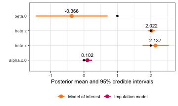
plot(framingham_model2.2)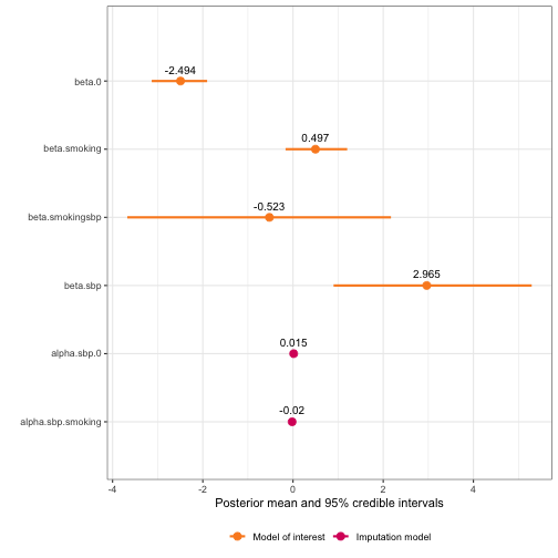
plot(framingham_model2.3)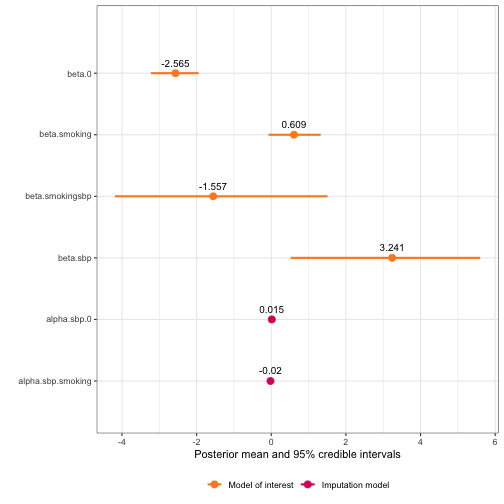
plot(framingham_model2.5)
framingham_model2.1$summary.hyperpar
#>                                                 mean       sd 0.025quant  0.5quant 0.975quant      mode
#> Precision for the Gaussian observations[2] 75.941763 3.694984 68.9643744 75.839341  83.509525 75.608321
#> Precision for the Gaussian observations[3] 19.900701 1.237511 17.5888076 19.857868  22.459486 19.763236
#> Beta for beta.smokingsbp                   -1.549041 1.354832 -4.1265836 -1.578576   1.205354 -1.708567
#> Beta for beta.sbp                           3.030323 1.193298  0.6201075  3.050937   5.317642  3.140323
framingham_model2.2$summary.hyperpar
#>                                                   mean       sd  0.025quant    0.5quant 0.975quant        mode
#> Precision for the Gaussian observations[2] 156.9883399 7.229709 143.1926400 156.8372549 171.652037 156.5682728
#> Precision for the Gaussian observations[3]  22.1572213 1.655540  19.0896008  22.0913348  25.604402  21.9514968
#> Beta for beta.smokingsbp                    -0.5231413 1.490996  -3.6739986  -0.4503943   2.171770  -0.1023884
#> Beta for beta.sbp                            2.9651518 1.117829   0.8996622   2.9228739   5.292024   2.7260210
framingham_model2.3$summary.hyperpar
#>                                                 mean       sd 0.025quant  0.5quant 0.975quant      mode
#> Precision for the Gaussian observations[2] 45.151167 2.190922 40.9948014 45.097007  49.619168 44.986819
#> Precision for the Gaussian observations[3] 19.176661 1.275318 16.7672718 19.141740  21.786114 19.087701
#> Beta for beta.smokingsbp                   -1.556773 1.452213 -4.1875780 -1.626083   1.507422 -1.956430
#> Beta for beta.sbp                           3.240676 1.294155  0.5215732  3.298372   5.600184  3.571394
framingham_model2.5$summary.hyperpar
#>                                                     mean           sd    0.025quant      0.5quant   0.975quant          mode
#> Precision for the Gaussian observations[2]  5.053238e-11 2.451925e-12  4.585460e-11  5.048081e-11 5.550617e-11  5.039490e-11
#> Precision for the Gaussian observations[3]  1.880235e+01 1.224319e+00  1.650633e+01  1.876300e+01 2.132478e+01  1.868547e+01
#> Beta for beta.smokingsbp                   -1.570571e+00 1.390761e+00 -4.317334e+00 -1.567547e+00 1.158593e+00 -1.555004e+00
#> Beta for beta.sbp                           3.234344e+00 1.245149e+00  7.929082e-01  3.230958e+00 5.695506e+00  3.216894e+00